The first image we will draw with the Watson Graphics Lab is a circle located in the center of the drawing window. In order to draw this circle using the lab’s interactive mode perform the following sequence of steps:
- Click the mouse on the Circle button to tell the system you wish to define a circle.
- Click the mouse in the center of the drawing area. This tells the environment where to place the center of the circle.
- Position the mouse where you would like the rim of the circle to be and press the mouse button once again.
The circle should now appear in the drawing window. You may also notice that as you created the drawing, some text appeared in the Variable Declarations and Program Code windows. This text is, in fact, a WGL program to create the same image you just drew interactively. To see that this is true, you could run the program by pressing the Run button. Run will clear the drawing window then execute the program code. An example program that draws a circle in the center of the drawing window is presented in Figure 6.10. The program created by the environment from your interactively produced drawing should be similar. It may not be identical, however, because the actual location and size of the circle you defined may be somewhat different from the one defined here.
We have now seen that the Watson Graphics Lab is capable of automatically generating a WGL program from an interactively drawn picture. But, how does one go about writing a program to draw a circle from scratch – without using the interactive drawing mode?
Before starting to write any program you must first determine exactly what you want to accomplish. For a WGL graphics program, you must decide the objects you wish to draw, such as circles, lines, or points; and then select the characteristics of these objects, such as their location, size, and color. Only after determining what needs to be done should you turn to the question of how to go about achieving the desired result.
Drawing Window
Variable Window
Program Code
Figure 6.10: A program that draws a circle in the center of the drawing window
In our current example, you may think the “what” question has already been satisfactorily answered. What we want to do is “draw a circle in the center of the drawing window”. This is only a partial answer. We need more detailed information. Where, exactly, is the center of the drawing window located? What size should the circle be? What color should be used to draw the circle?
A circle is generally specified by a center point and radius, as discussed in Sections 6.3 and 6.4. Since Watson’s drawing window coordinate system is defined from 0 to 299 in both the X and Y directions, the “center” of the drawing window is located at (150,150).[3] Hence, (150,150) should be the center point of the circle. Next, we must decide how big we want the circle to be. Let’s say we want the circle to be 100 units across (i.e., have a diameter of 100 units). Since radius is always ½ diameter, the radius value will be 50. This will produce a medium-sized circle in the 300 by 300 drawing window. For the moment, let’s say that we don’t really care what color “ink” will be used to draw this circle.
Now that we have specified more precisely “what” we want the program to do, we can turn to the question of “how” the program should go about achieving this goal.
First, we need to tell Watson to create a circle. This is done by clicking on the Circle button which produces the following statement in the variable declarations window:
circle c1
Watson has now created a variable called c1 of type circle. Nothing is yet drawn in the drawing window. Why? Well, one reason is that we have not yet described the size and location of the circle. In order to do this, we need to assign values to the circle variable with the assignment statement. Pressing the Assign button will cause the following generic assignment statement to appear in the program code window.
VARIABLE = EXPRESSION
Note that the words “variable” and “expression” are in upper case. Upper case is used by the Watson Graphics Lab to indicate a placeholder of a particular type. Clicking on “variable” will cause a popup box to appear which lists all of the currently valid choices for “variable”. In this example there is only one valid choice: c1. Selecting c1 and then clicking the “OK” button will cause “variable” to be replaced by c1. In addition, the form of the assignment statement will change so that it now looks like this:
c1 = (( X , Y ), RADIUS )
The reason for this change is that once Watson knows that the object you wish to assign a value to is a circle, it will automatically provide the appropriate expression type. A circle always consists of a center point (X,Y) and a radius RADIUS. Clicking on the X, Y, and RADIUS place holders will allow you to specify appropriate values. Replacing X with 150, Y with 150, and RADIUS with 50, will result in the following complete assignment statement. (You can tell it is complete, since there are no upper case place holders.)
c1 = ((150,150),50)
Now Watson knows about a circle called c1. It knows where the circle should be located and how big it should be. So what happens if you press the Run button in order to execute the program? Nothing! Why? The answer is that you never told Watson to actually draw the circle, so it didn’t. This can be rectified by adding a “draw” statement to the program. Here is the generic draw statement.
draw( OBJECT )
Once we select “object” and replace it with c1, we have the following:
draw(c1)
Draw is an output statement. It draws an object in the drawing window. The object must be completely defined before it can be drawn. In general, this means that an object must be declared in the variable declarations window and then be assigned a value by appearing on the left hand side of the “=” operator in an assignment statement before it can appear in a draw command.
Our program is now identical to the one given in Figure 6.10, which was created interactively. Clicking the “Run” button will cause a medium-sized circle to be drawn in the center of the drawing window.
So far, this example has introduced three very important programming concepts: variable declarations, assignment, and output. Many beginning students tend to confuse these three concepts, but they are actually quite distinct. Variable declarations, such as circle c1, define the objects that may be manipulated by the program. In general, an object must be defined before it can be manipulated. Assignment statements, such as c1 = ((150,150),50) place particular values into variables that have already been declared. In our graphics language, assignment statements are used to define the characteristics, such as location and size, of objects. Output statements, such as draw(c1), are used to display results. They actually cause objects to be drawn in the drawing window.
To continue with our example, let’s say that having seen the output of this program we decide that the circle should be somewhat larger. Specifically, let’s change the diameter of the circle from 100 to 150 units. Hence, the radius should be increased from 50 to 75 units. This is very simple to do in the Watson Graphics Lab. Click the mouse on the value of 50 in the assignment statement. A popup box will appear which will allow you to enter another constant, in this case 75. After entering 75 press the “OK” button. The program now has the following form:
- Variable Declarations
- circle c1
- Program Code
- c1 = ((150,150),75)
- draw(c1)
If you press the “Run” button, the drawing window will be cleared and the new, larger circle will be displayed.
Let’s make one more change to this example before moving on. The color that Watson draws with defaults to red. In other words, if you don’t specify a drawing color, Watson will choose red for you. Let us, instead, specify that the circle be drawn in green. This change is easily made by inserting a “color” statement before the draw statement. The color statement is equivalent to instructing Watson to pick up a pen of a particular color. Anything Watson draws after the color statement is encountered will be drawn in the specified color.
To insert a new statement in the program, click on (or just to the left of) the insertion symbol “ | ” at the beginning of the line on which you wish the insertion to take place. For this example, click on the “ | ” at the beginning of the draw(c1) line. You will notice that an insertion point symbol “ > ” now appears on an otherwise empty line directly above the draw command. The program code window now contains the following:
|o c1 = ((150,150),75)
>
|o draw(c1)
Clicking the “Color” button will place a “color” statement at the insertion point and then create a new insertion point on the line following that statement. Hence, the program code window will contain the following:
|o c1 = ((150,150),75)
|o color( COLOR_NAME )
>
|o draw(c1)
Next, the place holder “color_name” needs to be replaced with the color constant green. To do so, click on the “color_name” placeholder. A list of available colors will appear in a popup box. Select the color “green” and then press the “OK” button. Here is what the resulting program looks like.
|o c1 = ((150,150),75)
|o color(green)>
>
|o draw(c1)
Notice that the insertion point is still directly above the draw statement. This means that any new statements added to the program will be inserted between the color(green) and draw(c1) statements. The insertion point can be moved by clicking on the insertion symbol, “ | ”, on some other line of the program, or insertion can be “closed” by clicking on the insertion symbol anywhere below the last line of the program. When insertion is closed, all new statements are added to the end of the program. Since we do not wish to insert any more statements into the program at this time, we should close insertion.
Once insertion has been closed, our example program looks like this:
|o c1 = ((150,150),75)
|o color(green)
|o draw(c1)
You may now press the “Run” button to see the circle drawn with green ink. Pressing “Run” causes the following actions to take place. First, the center point and radius of circle c1, are set to (150,150) and 75, respectively. Second, the drawing color is set to green. Third, the circle c1 is drawn using the current drawing color, green. These actions will be taken in exactly the order indicated.
The order of statements in a program is very important. This is because computer languages depend on the concept of sequence. Sequence means that each statement is executed, or performed, in the order it is encountered in the program, starting at the first statement and proceeding to the last statement.
What if the statements of this program appeared in a different order? Say we decided to move the color statement so that it follows the draw statement. How could we accomplish this and what would be the effect of this change on the behavior of the program?
We have already seen how to insert statements into a WGL program using the insertion symbol “ | ”. It is also possible to delete WGL statements using the target symbol “ o ”. To remove a WGL statement from the program, first click on the target symbol to the left of that statement. The statement will be highlighted and a pop up confirmation box will appear. Press “OK” and the statement will be deleted.
In the current example, we want to move the color statement to the end of the program. While the Watson Graphics Lab does not directly support a “move” operation, the change can easily be achieved by (1) deleting the old color statement using the target symbol and then (2) inserting a new color statement at the end of the program. After making this change, the program will have the following form.
|o c1 = ((150,150),75)
|o draw(c1)
|o color(green)
Pressing “Run” will now cause: (1) the center point and radius to be assigned to the circle c1, as in the above example, (2) the circle to be drawn using the current drawing color, (3) the drawing color to be set to green. The result of this program is that a red circle will be drawn, since red is the default drawing color and the program draws the circle before changing the drawing color. Any draw commands appearing after the color(green) statement will be drawn using green “ink” – that is, until another color statement is encountered which changes the current drawing color yet again.
A more serious problem would occur if the assignment statement for c1 appeared after the draw statement for c1. The program would attempt to draw a circle before it had been told where to place the circle and how big it should be!
Watson tries to help you avoid some sequencing errors by preventing certain types of edit operations from taking place. For example, when specifying an “object” in the draw statement, Watson only presents those drawable objects that have already been assigned values. This helps prevent the kinds of errors in which the programmer attempts to draw an object before fully defining it. Be warned however, that while Watson can prevent you from making some simple mistakes, there are many errors it cannot prevent. When writing a program, you are “in charge”. Watson is just an assistant that tries to “help out” whenever it can.
At this point it is natural to ask yourself why you should learn to write WGL programs. After all, as demonstrated above, the Watson Graphics Lab can automatically write programs for you, so why should you bother to learn to produce them manually. This is a good question, and deserves a good answer. Here are three reasons why learning to write WGL programs is important:
- The programming approach gives you finer control over the image to be drawn by allowing you to specify the characteristics of objects very precisely. In our circle program we were able to specify the center of the circle as the exact center of the drawing window (150,150). It would be very difficult to place the circle in the exact center of the drawing window by hand using the interactive mode.
- Programs allow you to do some things, like animation, that are impossible to do interactively. As we will see in the next section of this chapter, Watson is capable of producing limited animation – images that appear to move – but only if the program mode is used. Animation involves quickly displaying a series of images one after another to simulate the visual appearance of movement. There is nothing in the interactive drawing mode of the Watson Graphics Lab that corresponds to this effect.
- Perhaps the most important reason for writing WGL programs is that by doing so you are learning many of the concepts that are used in the majority of programming languages. Few environments exist today that can write programs for you. The Watson Graphics Lab is an exception, not the rule. So, normally when a program is needed there is no choice but to develop it by hand. The languages professional programmers use, while more complex than WGL, share many of the same basic features, including: data types, variable declarations, assignment statements, output statements, and use of the sequence concept.
Next, I present a somewhat more complex static image and develop a program to draw that image. One feature of this program will be the creation of complex objects from simpler objects. The program will introduce the data types: point, line, and polygon. Distance will also be further explored. An annotated version of the image the program is to produce is presented in Figure 6.11. The numbers and text will not be in the final image, they are included here only for reference.
In order to construct a program to draw this image, we should first concentrate on the question of what we want to draw, then address the issues of how we will proceed. The “what” question is not as straight forward as it first appears, since there are many ways of describing the image of Figure 6.11. One could view the example image as simply a
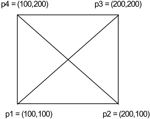
Figure 6.11: Box shaped polygon with two intersecting lines
collection of points arranged in a certain way. Another view is as six separate lines. The image may also be viewed as a box with two intersecting lines. All three of these views (and many others) are “correct” ways of describing what needs to be drawn.
However, all ways of viewing the problem are not equally appropriate, since the amount of work required to draw the image depends heavily on how one chooses to decompose it. For example, if we chose to view the image simply as a collection of points (which it is), we would end up creating a program with nearly six hundred draw commands – one for each point or pixel. Viewing the image as six lines (which it is) would result in a program with only six draw commands. Viewing it as a box with two intersecting lines results in a program with only three draw commands. Finding the “right” level of abstraction with which to describe an image is more an art than a science, but, in general, we want to decompose the image into a small number of relatively high-level components. For this reason we will view the image as a box with two intersecting lines.
Now that we have addressed the “what” question by decomposing the image into manageable parts, we need to address “how” we will actually go about drawing the image. One way to begin is to look at the end points of the lines and corners of the box, since these are the most important points – the ones we will use to define our polygon and lines. These points are labeled p1, p2, p3, and p4 in Figure 6.11. The point p1 is located at (100,100), p2 is at (200,100), p3 is at (200,200), and p4 is at (100,200). This information can be expressed in WGL as follows:
- Program Declarations
- point p1 p2 p3 p4
- Program Code
- p1 = (100,100)
- p2 = (200,100)
- p3 = (200,200)
- p4 = (100,200)
However, this is probably not the best way to proceed. Entering constants in WGL can be somewhat tedious since you must enter each digit on a “graphical keypad”.[4] Another reason to avoid over reliance on constants is that programs written with a large number of constants are not very flexible. Making even small changes can result in a lot of work. For example, say we decided that our box and line need to be moved to another location on the screen. To implement such a change would involve modifying all eight of the distance constants shown above; a somewhat lengthy and error prone task.
A better way of implementing the points presents itself when you realize that the program actually uses only two distinct distance values: 100 and 200. Explicitly defining two distance variables and then using them to define the points leads to a much more flexible program, as well as one that can actually be entered more quickly, despite the fact that it appears longer. Incorporating this modification leads to the following program fragment. (It’s only a fragment, since the program is not yet finished.)
- Program Declarations
- distance d1 d2
- point p1 p2 p3 p4
- Program Code
- d1 = 100
- d2 = 200
- p1 = (d1,d1)
- p2 = (d2,d1)
- p3 = (d2,d2)
- p4 = (d1,d2)
Now that the underlying points have been defined, the lines and polygon which are based on them can be specified. An inspection of Figure 6.11 indicates the location of the endpoints of the lines but it does not specify which ones should be the starting points and which should be the ending points. Arbitrarily, line l1 will be defined as starting at point p1 and ending at point p3. Similarly, line l2 will be defined as starting at point p2 and ending at point p4. These lines can be coded in WGL as follows:
l1 = (p1,p3)
l2 = (p2,p4)
Note that I could just as easily have reversed the start and end points of these lines (e.g., defined l1 as starting at p3 and ending at p1).
Next, I define the box using a polygon. As described earlier, polygons are composed of connected lines, where the end point of the last line is the same as the start point of the first line. In order to define our box, we need to select a starting point and decide whether to trace out the box in a clockwise or counter-clockwise direction. Since these choices will not affect the look of the finished image (only the manner in which it is drawn), I arbitrarily choose the lower left hand corner of the box, point p1, and the counter-clockwise direction. Hence, the box may be defined as follows:
g1 = (p1, p2, p3, p4, p1)
This statement implicitly defines lines from p1 to p2, from p2 to p3, from p3 to p4, and from p4 back to p1.
Drawing Window
Variable Window
Program Code
Figure 6.12: A complete program that generates the image of Figure 6.11
The final step is simply to draw the two lines, l1 and l2, and the box, g1.
draw(l1)
draw(l2)
draw(g1)
The order of these draw statements will not affect the look of the final image. A complete program for generating the image of Figure 6.11 appears in Figure 6.12.
Before leaving this example, I want to reemphasize two concepts. First, it really did not matter that I decided to define the lines first and then the box. I could just as easily have chosen to define the box first and then the lines; or even defined one of the lines, then the box, then the other line. The reason that order is unimportant here is that the lines and box are independent of one another – the definition of the box does not refer to the lines and vice versa. Keep in mind however, that it is extremely important for the distances to be defined before the points and for the points to be defined before the lines and box, since the lines and box are defined using points and points are defined using distances.
The second concept relates to flexibility. This program is quite flexible due to the fact that complex objects are defined in terms of simpler objects which are, in turn, defined using only two distance constants, 100 and 200. The location and/or the size of the image can be modified by changing the values stored in d1 and d2. For example, you can move the image from the center of the drawing area towards the upper right hand corner by changing d1 from 100 to 150 and d2 from 200 to 250. Similarly, you can make the image larger by changing d1 from 100 to 50 and d2 from 200 to 250. These tasks would be much more difficult if the points had been directly defined in terms of distance constants.
Footnotes
[3] Actually, the exact center of this drawing area would be at (149.5, 149.5) which falls between pixels. Rounding up to the nearest pixel gives (150, 150).
[4] Having designed this lab, I obviously think that the keypad is a good idea. It prevents you from entering the wrong kind of data, such as letters when a number is needed. But, I acknowledge that using the keypad is slower than typing.